1 About
This is a supplementary analysis file for the article “The flying bomb and the actuary” published in Significance (October 2019).
The Significance article tells the story of our attempt to recreate a paper by R. D. Clarke from 1946 showing that V-1s falling on London followed a Poisson distribution. The article details the data cleaning and analysis we carried out in R on a dataset of V-1 and V-2 impacts on London, compiled from photographs of the original London County Council bomb damage maps published by the London Metropolitan Archives. For more information on the V-1 and V-2 bombs, see Wikipedia.
The purpose of this document is:
- to reproduce the analysis covered in the article.
- to act as a guide for those looking to do further exploration of the dataset.
Disclaimers:
- We are not experts in spatial statistics, so this is quite a basic analysis.
- There may be mistakes, as this document is deliberately a “show your working”. Constructive criticism is very welcome!
- Code: in general, we have used the tidyverse i.e. the preferred format for data is a tibble. However, there is no enforcement of tidyverse rules and the code sometimes switches to base R when it seems most convenient.
Please feel free to get in touch with errors/comments/questions: you can email us at liam [dot] philip [dot] shaw [at] gmail.com and luke [dot] francis [dot] shaw [at] gmail.com. We are also (Liam, Luke) on Twitter.
2 Data import and clean
All packages required:
library(rgdal)
library(ggforce)
library(tidyverse)
library(geosphere)
library(remotes)
remotes::install_github("geotheory/londonShapefiles")
## * checking for file 'C:\Users\Luke\AppData\Local\Temp\RtmpEXFvc4\remotes3270e957772\geotheory-londonShapefiles-7938344/DESCRIPTION' ... OK
## * preparing 'londonShapefiles':
## * checking DESCRIPTION meta-information ... OK
## * checking for LF line-endings in source and make files and shell scripts
## * checking for empty or unneeded directories
## * building 'londonShapefiles_1.0.tar.gz'library(maptools)
library(concaveman)
library(mclust)
library(DT)First we read in the data. The file “bomb_map.kml” is the downloaded file from the Google Maps layer with the impacts, stored in the appropriate directory. There may be a nifty way to directly read from the url directly.
vones = readOGR(dsn = "bomb_map.kml", layer = "V1")
vones = as_tibble(vones)
#give sensible column names
colnames(vones)[colnames(vones)=="coords.x1"] <- "long"
colnames(vones)[colnames(vones)=="coords.x2"] <- "lat"
The analysis we are doing focuses on the distance between points. Latitude and longitude are not ideal for this, as they represent angles. Moving one degree in a direction can result in a great deal more movement than in another, depending on the location on the Earth’s surface. Instead, we need a spatial reference system. We chose to convert to the Ordnance Survey standard British National Grid, in which the Eastings and Northings have units in metres. This means we can use traditional euclidean geometry to estimate distance between points. We found the code to do this here.
#initially in latitude, longitude
cord.dec = SpatialPoints(cbind(vones$long, vones$lat), proj4string=CRS("+proj=longlat"))
#UK epsg https://spatialreference.org/ref/epsg/osgb-1936-british-national-grid/
cord.UTM <- sp::spTransform(cord.dec, CRS("+init=epsg:27700"))
## Warning in showSRID(uprojargs, format = "PROJ", multiline = "NO"): Discarded
## datum OSGB_1936 in CRS definition#add BNG to vones dataset
vones$easting = cord.UTM$coords.x1
vones$northing = cord.UTM$coords.x2
#tidy up
vones = dplyr::select(vones,c("Description", "easting","northing"))For plotting, we want something to give an impression of location within London. We could use rasters and maps, but the simplest solution is to include the River Thames (as anybody who’s seen Eastenders will know). Thanks to geotheory for the shapefile!
londonShapefiles::load_thames()  # River Thames
#strip away all but essential info - our plotting needs are simple
thames_line = thames@polygons[[1]]@Polygons[[1]]@coords
thames_line = thames_line %>%
  tibble::as_tibble() %>%
  dplyr::rename(easting=V1,northing=V2) %>%
  dplyr::filter(easting>520000,easting<550000)
Now we can create an initial plot with the V-1 bomb locations and the Thames.
base_plot = ggplot(data=vones, aes(x=easting, y=northing)) +
  coord_fixed() +
  theme_bw() +
  geom_point() +
  geom_polygon(data=thames_line, alpha=1, aes(col = 2, fill = 2)) +
  theme(legend.position = "none")
base_plot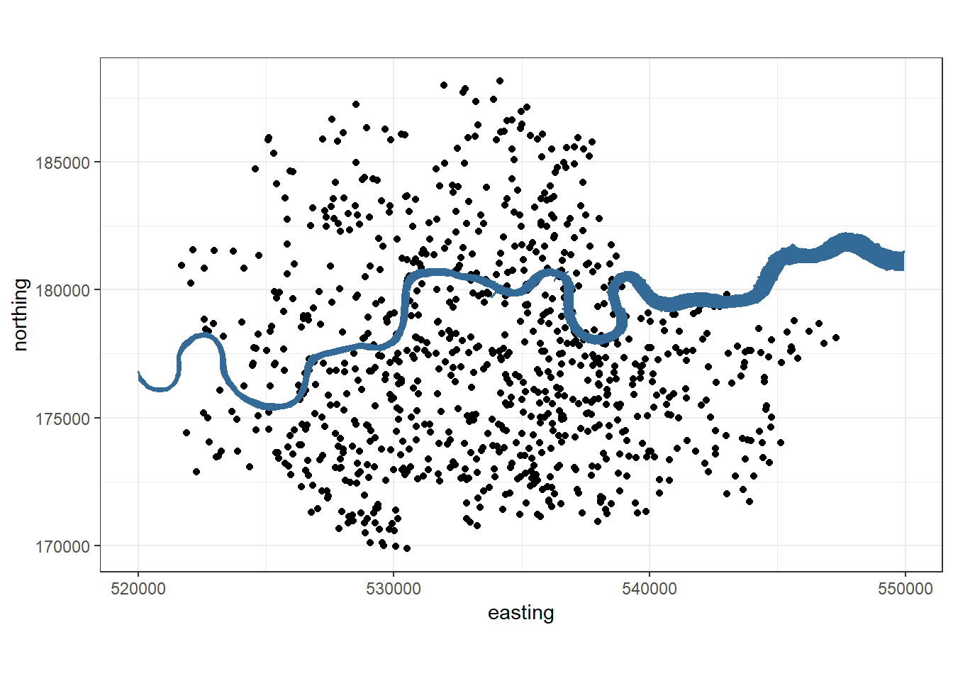
3 Replicating Clarke
3.1 The Grid
Clarke is not specific about the exact location of his grid that he chose. Here the things we knew about the area:
- Made of 576 squares, each with width 0.25km\(^2\)
- 537 V-1 bombs fallen inside it
- In “south London”
- (probably) follows BNG lines, as Clarke would have been using standard British maps
We’re not sure whether the London County Council maps contain the whole area that Clarke used. So we choose a reasonable area that contains 532 V-1s (not 576) and fitted all the other criteria.
#The boundaries were chosen to have same dimensions a clarke and to
#have roughly the same number of bombs in
xmin = 525000
xmax = 543000
ymin = 172000
ymax = 180000
base_plot+geom_rect(xmin=xmin, xmax=xmax,
                    ymin=ymin, ymax=ymax,
                    alpha=0.1, fill=NA, colour="red", size=0.5)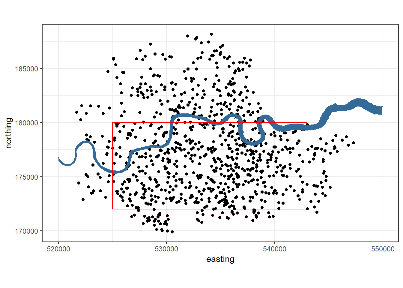
Now we have the grid, we can replicate the analysis to get the same contingency table as Clarke.
3.2 Mirroring Clarke, with a chi-squared warning?
#cutout just the bombs inside the rectangle
vones_region <- vones[which(vones$easting>xmin & vones$easting<xmax &
                              vones$northing>ymin & vones$northing<ymax),]

# Table up the counts
step = 500
nrow_x = (xmax-xmin)/step
ncol_y = (ymax-ymin)/step
total_squares <- (nrow_x * ncol_y)
hits_matrix <- matrix(nrow = nrow_x, ncol=ncol_y)
for (i in seq(1, nrow_x)){
  for (j in seq(1, ncol_y)){
    hits_matrix[i, j] <- nrow(vones_region[which(vones_region$easting>xmin+step*(i-1) &
                                                   vones_region$easting<xmin+step*i &
                                                   vones_region$northing>ymin+step*(j-1) &
                                                   vones_region$northing<ymin+step*j),])
  }
}
# Lambda
lambda <- nrow(vones_region) / total_squares

# Replicate Clarke
comparison_df <- data.frame(num_bombs_per_square = 0:4,
                            poisson = sapply(seq(0, 4),
                                             function(x) dpois(x, lambda)*total_squares),
                            actual = as.numeric(table(hits_matrix)[1:5]))
comparison_df <- rbind(comparison_df,
                       data.frame(num_bombs_per_square = "5 and over",
                                  poisson = 576-sum(comparison_df$poisson),
                                  actual = as.numeric(table(hits_matrix))[6]))
# Chi-squared test
chisq.test(comparison_df[c('poisson','actual')])
## Warning in chisq.test(comparison_df[c("poisson", "actual")]): Chi-squared
## approximation may be incorrect##
## Pearson's Chi-squared test
##
## data: comparison_df[c("poisson", "actual")]
## X-squared = 0.64365, df = 5, p-value = 0.9859Hold on a second, what’s that error: “Chi-squared approximation may be incorrect”?
It turns out it’s because we have small categories, namely the “5 and over” row. One change could be to simulate the values instead (the function has a “simulate.p.value” parameter), but this will still be inconsistent due to the small numbers in the table. All that matters for the narrative is that the p-value is always large, which shows the columns are similar and hence we have no reason to reject the hypothesis that the bombs fell at random in the area chosen. But as a statistician this is still unsatisfying.
3.3 Copying Clarke exactly
Clarke quotes some of his intermediate results in his paper:
Applying the \(\chi^2\) test the comparison of actual with expected figures, we obtain \(\chi^2 = 1.17\). There are 4 degrees of freedom, and the probability of observing this or a higher value of \(\chi^2\) is .88
#numbers from his paper
clarke_df = data.frame(num_bombs_per_square = 0:4,
                       poisson = 576*dpois(x=0:4, lambda = 537/576),
                       actual = c(229,211,93,35,7))
clarke_df = rbind(clarke_df,
                  data.frame(num_bombs_per_square = 5,
                             poisson = 576-sum(clarke_df$poisson),
                             actual = 1))
#doing step-by-step
clarke_df$test_stat_components = (clarke_df$actual - clarke_df$poisson)^2 / clarke_df$poisson
clarke_test_stat = sum(clarke_df$test_stat_components) #1.17
clarkes_pvalue = pchisq(clarke_test_stat, df = 4, lower.tail=FALSE)
print(paste('We recreate Clarke\'s p-value as ', clarkes_pvalue, '(he says .88)'))
## [1] "We recreate Clarke's p-value as 0.883150518919159 (he says .88)"3.4 … Is there a mistake?
We get the same warning as previously when using his table (not shown). So we can replicate Clarke’s example, but…you may be wondering, shouldn’t there be 5 degrees of freedom, not 4? When first shown the chi-squared test you learn the rule that the degrees of freedom is \((number\ of\ rows\ - 1) * (number\ of\ columns - 1)\) which here is \((6-1)*(2-1)\) = 5. Thinking in terms of what “degrees of freedom” means, this makes sense: when you get to the last row the numbers are fixed as we know both columns add to 256.
So did Clarke get it wrong? We were pretty certain the answer was “yes”, as this blog and the main article initially claimed. But the real answer is “no”, and we are thankful to Erik Holst for this correction. The reason 4 degrees of freedom is correct is that a parameter had been estimated during the table creation - the lambda value used in the calculation of the expected number of squares. Thus we have lost another degree of freedom: \(6 - 1 - 1 = 4\).
Whatever permutation of the degrees of freedom and method we use, the p-value is always large, so the narrative is untouched. The distribution of V-1 impacts is well-described by a Poisson distribution.
4 “Spherical Clarke” - Random Sampling
We had the idea of using a more modern technique: randomly sampling a point and counted the bombs within a certain distance from it. Whereas Clarke dealt with a grid of squares, this techniques means dealing with circles (defined by a point and a radius).
To get a comparable lambda estimate to Clarke’s \(537/576 \approx 0.93\), we need to use the same area. Clarke’s estimate is the number of bombs falling in a 0.25km square. To map this to circles and find the radius we need to only use our trusty circle area formula \(area = \pi r^2\). Note how tricky this would be to do in latitude/longitude coordinates, however, in BNG easting/northing the units are metres so we can easily calculate our necessary radius:
\[r = \sqrt{500^2 / \pi} = \sqrt{250000 / \pi} = 282.094... \approx 282m\]
Now we have our circle radius we can copy Clarke’s methodology using circles instead of squares. We can also re-sample from circles already covered, sampling with replacement. Clarke was limited by physical map paper, but we can simulate as many times as we want!
Simulation approach:
- n times:
- randomly pick a location (x,y)
- count the number of bombs that landed within the circle with centre (x,y) and area 0.25km^2
- calculate the rate of bomb hits (our lambda estimate in Poisson terms)
This is a simple form of bootstrapping. Some further work could be to bootstrap to find the standard error in our final lambda estimate, as described by Jodie Burchell here.
4.1 A border for our data
We have the issue of not easily knowing the exact border of our data. We know that V-1 bombs fell outside of the data we have, as our data is only for the area is the County of London, which no longer exists. Because this area was in use over 70 years ago we couldn’t easily find a ready-made shapefile online!
A fix is to look at creating a hull, which is a polygon that covers our set of points. We can have: a convex hull, which is too bloated; a concave hull, which is too jagged; or a 'Goldilocks hull', which is 'just right' (sorry…).
#most simple hull - a rectangle defined by furthest bomb points
min_e = min(vones$easting)
max_e = max(vones$easting)
min_n = min(vones$northing)
max_n = max(vones$northing)
rectangle = tibble(easting =  c(min_e, min_e, max_e, max_e, min_e),
                   northing = c(min_n, max_n, max_n, min_n, min_n))

#convex (bloated) hull
convex = concaveman::concaveman(cbind(vones$easting, vones$northing), concavity = 10000)
convex = convex %>% as_tibble() %>% rename(easting=V1,northing=V2)

#concave (tight) hull
concave = concaveman::concaveman(cbind(vones$easting, vones$northing), concavity = 1)
concave = concave %>% as_tibble() %>% rename(easting=V1,northing=V2)

#conmid (goldilocks) hull
conmid = concaveman::concaveman(cbind(vones$easting, vones$northing), concavity = 2)
conmid = conmid %>% as_tibble() %>% rename(easting=V1,northing=V2)

hulls = rbind(cbind(rectangle, type="rectangle"),
              cbind(convex,type="convex"),
              cbind(concave,type="concave"),
              cbind(conmid,type="goldilocks"))
hulls = mutate(hulls, type = as.character(type))
hulls = as_tibble(hulls)

#why doesn't this work?
#base_plot + geom_path(data = hulls, aes(colour=type))

hulls_plot = ggplot(vones, aes(x=easting, y=northing)) +
  geom_point() +
  geom_path(data = hulls, aes(colour=type)) +
  theme_bw() +
  ggtitle('Candidate hulls for our boundary')
hulls_plot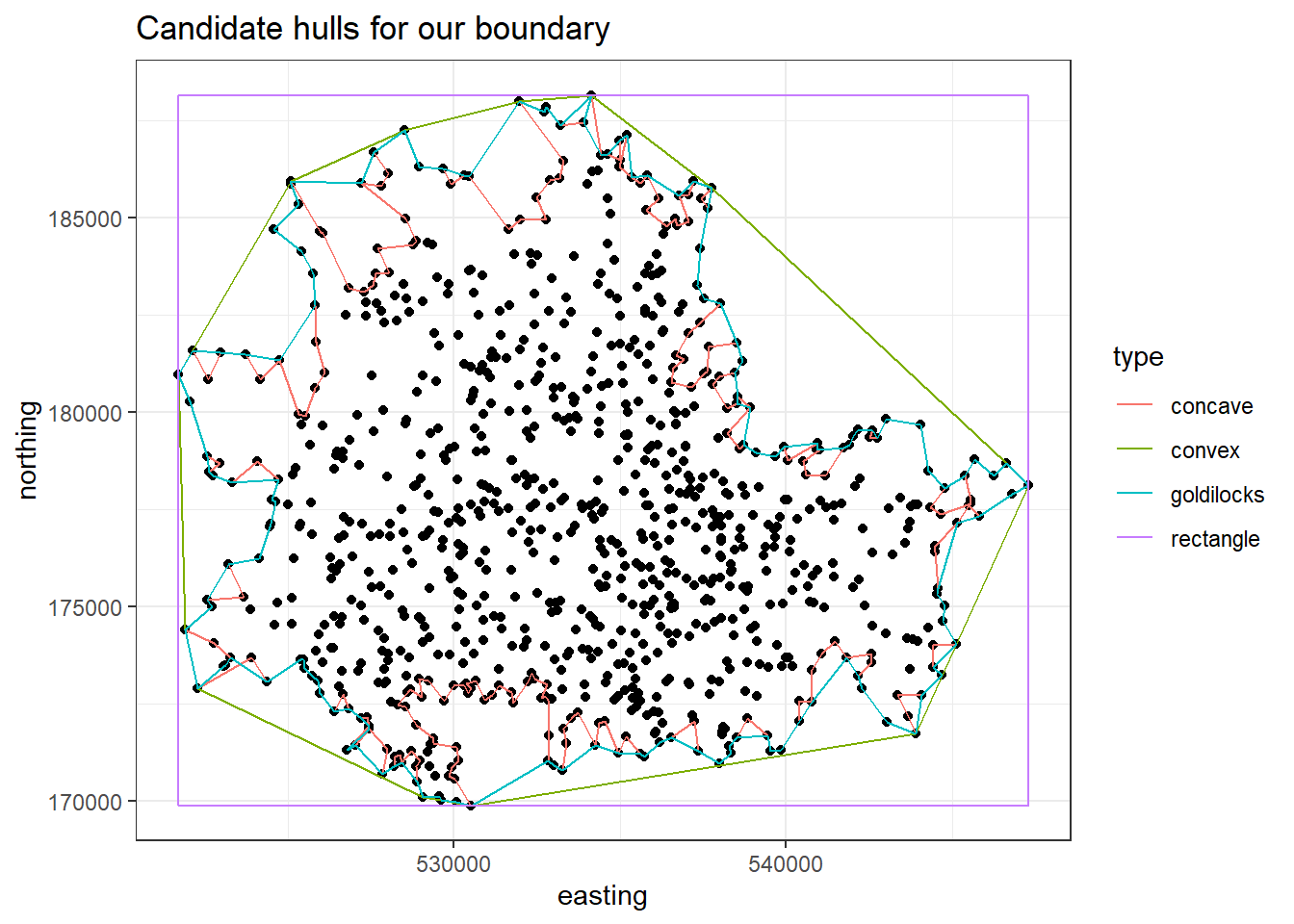
If we pick a hull that’s too large, we expect underestimate the bomb rate as we’ll have more arbitrary zeros, and if we pick a hull that is too small the reverse will happen.
vone_boundary_plot = ggplot(data=vones, aes(x=easting, y=northing)) +
  coord_fixed() +
  theme_bw() +
  theme(panel.grid = element_blank()) +
  geom_polygon(data=thames_line, alpha=1, aes(col = 2, fill = 2)) +
  geom_path(data = hulls %>% filter(type=='goldilocks'), colour='darkgrey', size = 2) +
  geom_point() +
  theme(legend.position = "none") +
  ggtitle('\"conmid\" (goldilocks) is chosen as the preferred boundary')
vone_boundary_plot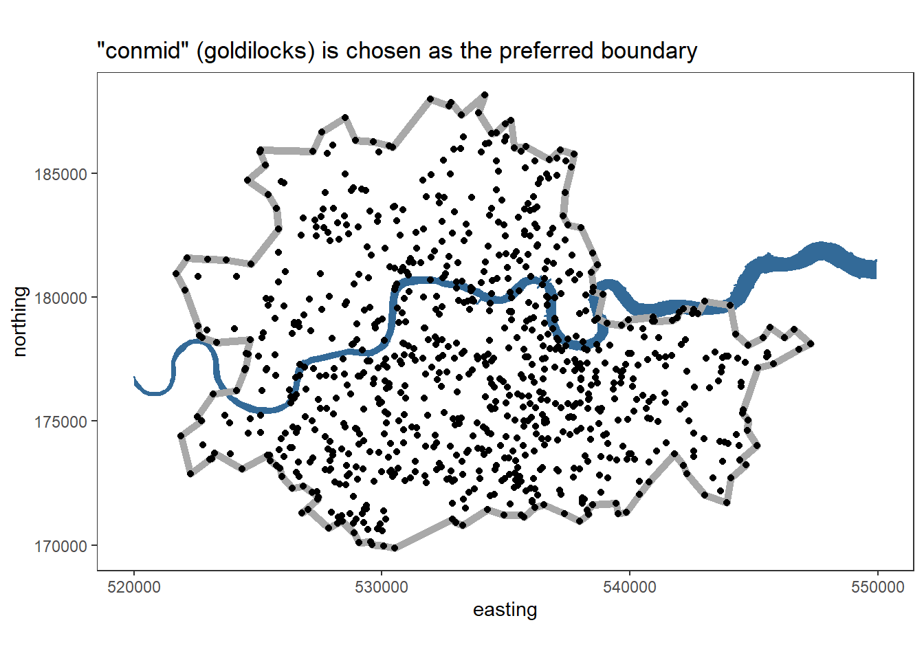
4.2 Creating the simulation
Our simulation approach now has a vital new step:
- n times:
- randomly pick a location (x,y)
- check the circle of area \(0.25km^2\) centre (x,y) is inside the hull. If not, try again
- count the number of bombs that landed within the circle with centre (x,y) and area \(0.25km^2\)
- calculate the rate of bomb hits (our lambda estimate in Poisson terms)
We need a few sub-functions for this process:
###Function for checking the circle is in the hull:

circle_inside_hullEN = function(centre, radius, hull){
  #given the centre and radius of a circle, output TRUE if the circle
  #is entirely inside the hull, and FALSE if not
  if(!identical(names(centre),c("easting", "northing"))){
    stop("centre names must be c(\"easting\",  \"northing\") in that order")
  }

  #take 360 points on the circle, then we'll individually check if inside the hull
  circle_points = tibble::tibble(easting = centre[1] + radius * cos(1:360),
                                 northing = centre[2] + radius * sin(1:360))
  inside = sp::point.in.polygon(point.x = circle_points$easting,
                                point.y = circle_points$northing,
                                pol.x = hull$easting, pol.y = hull$northing)
  return(all(inside!=0))
}

###Function for counting the number of bombs inside the circle:

count_hitsEN <- function(data, radius, centre){
  # function to check if a point is inside the circle, in Easting / Northing defn
  if(centre[1] < 500000 | centre[2] > 190000){
    stop("centre not in format (easting,northing)")
  }
  #function to return TRUE/FALSE for statement "point is inside circle"
  inside = function(easting, northing){
    return( (easting-centre[1])^2 + (northing-centre[2])^2 < radius^2 )
  }
  # run on all bombs
  bomb_count <- data %>%
    as_tibble() %>%
    mutate(inside=inside(easting, northing)) %>%
    filter(inside==TRUE) %>%
    count()
  return(bomb_count$n)
}

###Function for sampling circles and counting the number of bombs within them:

sample_n_circles = function(data=vones,
                            n = 1000,
                            hull = conmid,
                            r = sqrt(500^2 / pi),
                            max_attempts = 10000,
                            seed=1729){
  #Sampling the number of points within n random circles radius r that are
  #inside the hull

  num_outside_hull = 0 #for keeping track of bad circles
  set.seed(seed)

  #initialise our output data set
  valid_centres <- as_tibble(data.frame(matrix(nrow=0,ncol=3)))
  colnames(valid_centres) <- c("easting", "northing", "num_bombs")

  #loop through
  i = 1
  while(i < max_attempts){
    #randomly choose a point for centre of circle
    rx = runif(1, min_e, max_e)
    ry = runif(1, min_n, max_n)
    centre = c(rx,ry)
    names(centre) = c("easting","northing")

    #check if inside our hull - if so we'll check the number of bombs inside it
    if(circle_inside_hullEN(centre,r,hull)){
      valid_centres = bind_rows(valid_centres,
                                tibble(easting=centre[1],
                                       northing=centre[2],
                                       num_bombs=count_hitsEN(data, r, centre)))
    } else {
      num_outside_hull = num_outside_hull + 1
    }
    if(dim(valid_centres)[1]==n){
      #break the loop as we've sampled enough
      i = max_attempts+1
    } else{
      i = i + 1
    }
  }
  if(i==max_attempts){
    warning(paste("only got",
                  dim(valid_centres)[1],
                  " circles sampled, try changing hull or increasing max_attempts"))}
  return(valid_centres)
}
Now we can sample away:
s_rectangle = sample_n_circles(hull=rectangle)
s_convex = sample_n_circles(hull=convex)
s_conmid = sample_n_circles(hull=conmid)
s_concave = sample_n_circles(hull=concave)
We can also get our equivalent lambda to compare to Clarke - notably smaller than his estimate of around 0.93. This is because North London has a lower density of bomb hits.
lambda_from_hits = function(valid_centres){
  freq_tab = valid_centres %>% group_by(num_bombs) %>% count()
  sum(freq_tab$num_bombs*freq_tab$n)/sum(freq_tab$n)
}
#we'd expect the lambda to go biggest to smallest: I think
#it doesn't as we were just "unlucky" with there being zeros
#in the random selection that conmid never got to but concave
#did - note consistent seed in sample_n_circles function
lambdas = purrr::map(list(s_rectangle, s_convex, s_conmid, s_concave),
                     lambda_from_hits)
areas = unlist(purrr::map(list(rectangle, convex, conmid, concave),
                          function(x) sp::Polygon(x)@area[[1]]))
names(lambdas) = c('s_rectangle', 's_convex', 's_conmid', 's_concave')
DT::datatable(data.frame(shape = c('rectangle', 'convex', 'conmid', 'concave'),
                         area = round(areas/1000),
                         lambda  = unlist(unname(lambdas))),
              colnames = c('Bounding shape', 'area (km)',
                           'lambda (mean no. of bombs per circle during simulation)'))
Intuitively the area gets smaller as the shape does! The lambda value also gets smaller, which makes sense thinking about the fact the tighter the shape the fewer zero counts there will be, hence a larger lambda estimate. The fact that concave has very slightly higher rate than conmid is down to sampling chance - they are practically the same shape.
4.3 Perform the test
Now we have our sample we can get to our equivalent of Clarke’s contingency table but for the circles bootstrapping method.
total_circles <- dim(s_conmid)[1]
lambda <- sum(s_conmid$num_bombs) / total_circles
lambda
## [1] 0.761circle_comp_df <- data.frame(num_bombs_per_square = 0:4,
poisson = sapply(seq(0, 4), function(x)
dpois(x, lambda)*total_circles),
actual = as.numeric(table(s_conmid$num_bombs)[1:5]))
circle_comp_df <- rbind(circle_comp_df,
data.frame(num_bombs_per_square = "5 and over",
poisson = total_circles-sum(circle_comp_df$poisson),
actual = 0))
circle_comp_df## num_bombs_per_square poisson actual
## 1 0 467.198994 496
## 2 1 355.538435 319
## 3 2 135.282374 126
## 4 3 34.316629 46
## 5 4 6.528739 13
## 6 5 and over 1.134829 0# Chi-squared test
chisq.test(circle_comp_df[c('poisson','actual')])## Warning in chisq.test(circle_comp_df[c("poisson", "actual")]): Chi-squared
## approximation may be incorrect##
## Pearson's Chi-squared test
##
## data: circle_comp_df[c("poisson", "actual")]
## X-squared = 8.1489, df = 5, p-value = 0.1482Note the p-value is smaller than before.
4.4 P-hackers?
In the published article we state a p-value of 0.02 from the simulation (Figure 3). This p-value of 0.1568 is, of course, different. With simulations, the value depends very much on the simulated data, which is 1000 randomly simulated points. One could argue we have effectively performed p-hacking with simulations, and just chose the best interpretation, but this honestly is not the case! For one thing, we were very careful not to use the 0.05 traditional statistical rule in the main article, focussing instead on the interpretation of the p-value. We do not have the exact code and seed from when the original p-value was written, which for context was months prior to when we got around to writing this document, but it seems we got lucky and found a lower p-value than in this document.
However, this does highlight the fact that p-values are quite problematic. If we repeat our simulation 100 times, your intuition might be that the p-values should be similar…but that’s far from the case!
#set up the data frame with the known p-value
pvals_df = tibble(seed = 1749,
                  pval = 0.1568)

for (i in 1:100){
  #sample using seed i
  s_conmid = sample_n_circles(hull=conmid, seed = i)
  total_circles <- dim(s_conmid)[1]
  lambda <- sum(s_conmid$num_bombs) / total_circles
  circle_comp_df <- data.frame(num_bombs_per_square = 0:4,
                               poisson = sapply(seq(0, 4),
                                                function(x) dpois(x, lambda)*total_circles),
                               actual = as.numeric(table(s_conmid$num_bombs)[1:5]))
  circle_comp_df <- rbind(circle_comp_df,
                          data.frame(num_bombs_per_square = "5 and over",
                                     poisson = total_circles-sum(circle_comp_df$poisson),
                                     actual = 0))
  # Chi-squared test
  test = chisq.test(circle_comp_df[c('poisson','actual')])
  #add to data frame
  pvals_df <- tibble::add_row(pvals_df, seed=i,pval=test$p.value)
}
ggplot(data=pvals_df,mapping=aes(x=pval)) +
geom_histogram(breaks = seq(0,1,0.05)) +
labs(title = 'p-values for 101 simulations of 1000 points')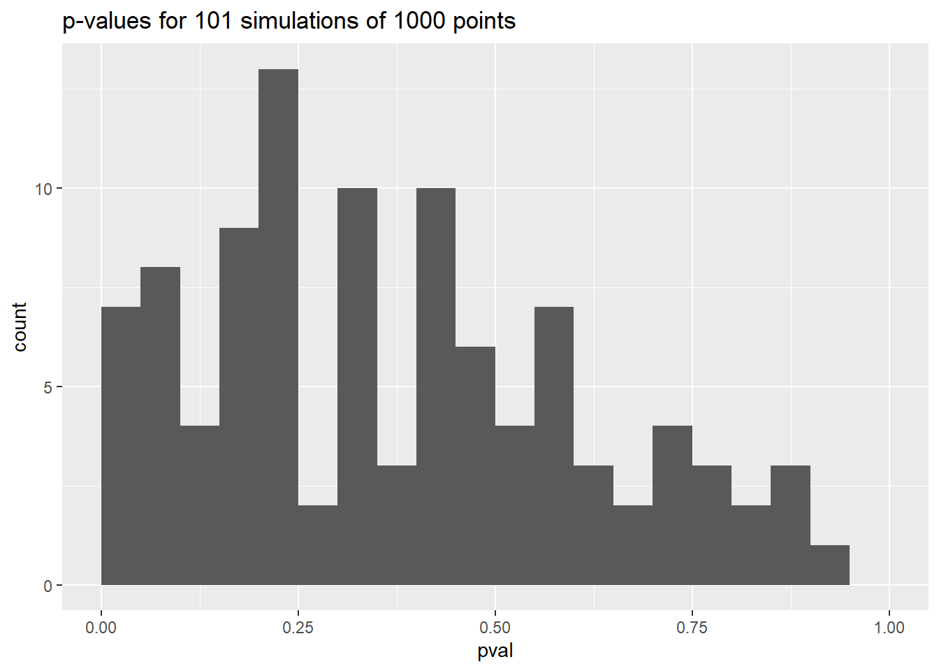
Although there is a peak in the distribution, possible p-values range from very small to quite large. This isn’t an original observation, but it should be a reminder about the trickiness of using p-values. Clarke’s example is popular in textbooks precisely because it’s quite rare to test a fit to a Poisson distribution with a Chi-squared test in such a convincing way.
5 Bomb Density
An assumption in the Poisson model is that the underlying distribution is uniform. That is to say, anywhere across the London area we have data for, the probability of a V-1 falling is constant. Depending on how you look at it, this may or may not be a fair assumption. On the one hand, of the 10,486 bombs launched by Germany, only 2,420 (23%) fell inside the London Civil Defence Region (source). One reason for this is many bombs fell outside of London, and a high variance would lead to fairly constant probability throughout London. On the other hand, it seems obvious central London would fare worse, and as the bombs were primarily fired from France you would assume south of the centre would get hit more than the north.
A Gaussian Mixture model can be used to assess if the underlying distribution is made up of one or more normal distribution. We can look to see if the model picks a centre close to Tower Bridge:
gmmod <- mclust::densityMclust(vones %>% select(easting,northing))
#Note the optimal model selected by BIC criterion involves 3 Gaussians.
plot(gmmod, what='density', type = 'hdr',
     data = select(vones, easting,northing), points.cex=0.5)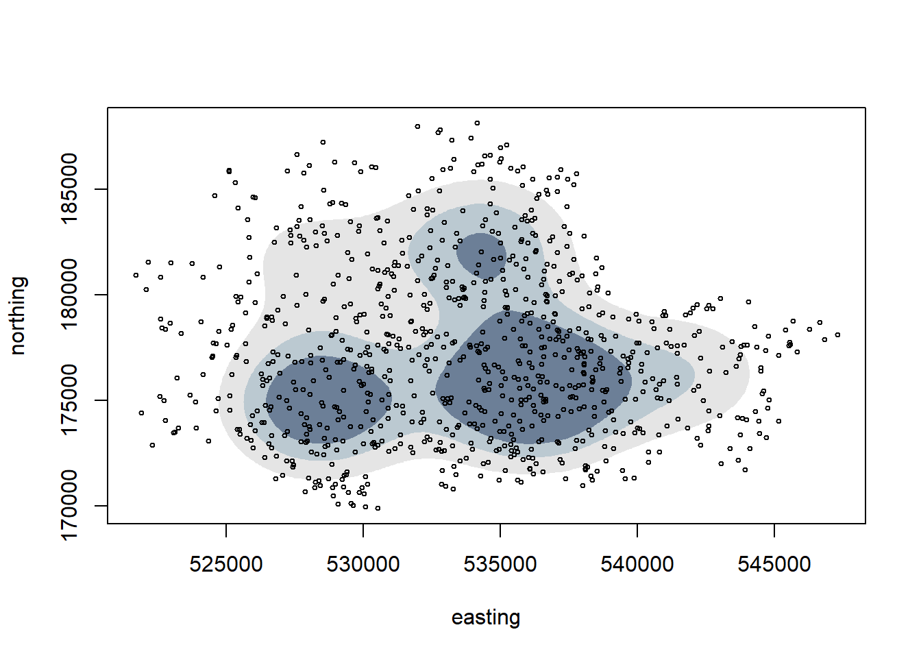
We can see that 3 Gaussians are selected as the best estimate, so that doesn’t necessarily fit the centred at Tower Bridge assumption. Note a boundary hasn’t been enforced in this method, which may bring the validity of the result into question.
For a more sophisticated use of mixture modelling, you might want to read this paper (July 2019, published after we wrote our article), which analyses the distribution of V-2s over time.
6 Conclusions
This document hopefully fills some of the gaps as to how we went about performing the analysis for this project. Feel free to get in touch if anything isn’t clear.
If you plot our equivalent of Clarke’s rectangular region, it looks like the night sky.
stars_df = data.frame(vones_region$easting, vones_region$northing)
plot(stars_df, xaxt='n', yaxt='n', ann=FALSE)
rect(par("usr")[1],par("usr")[3],par("usr")[2],par("usr")[4],col = "black")
points(stars_df, col='white', pch=19, cex=0.2)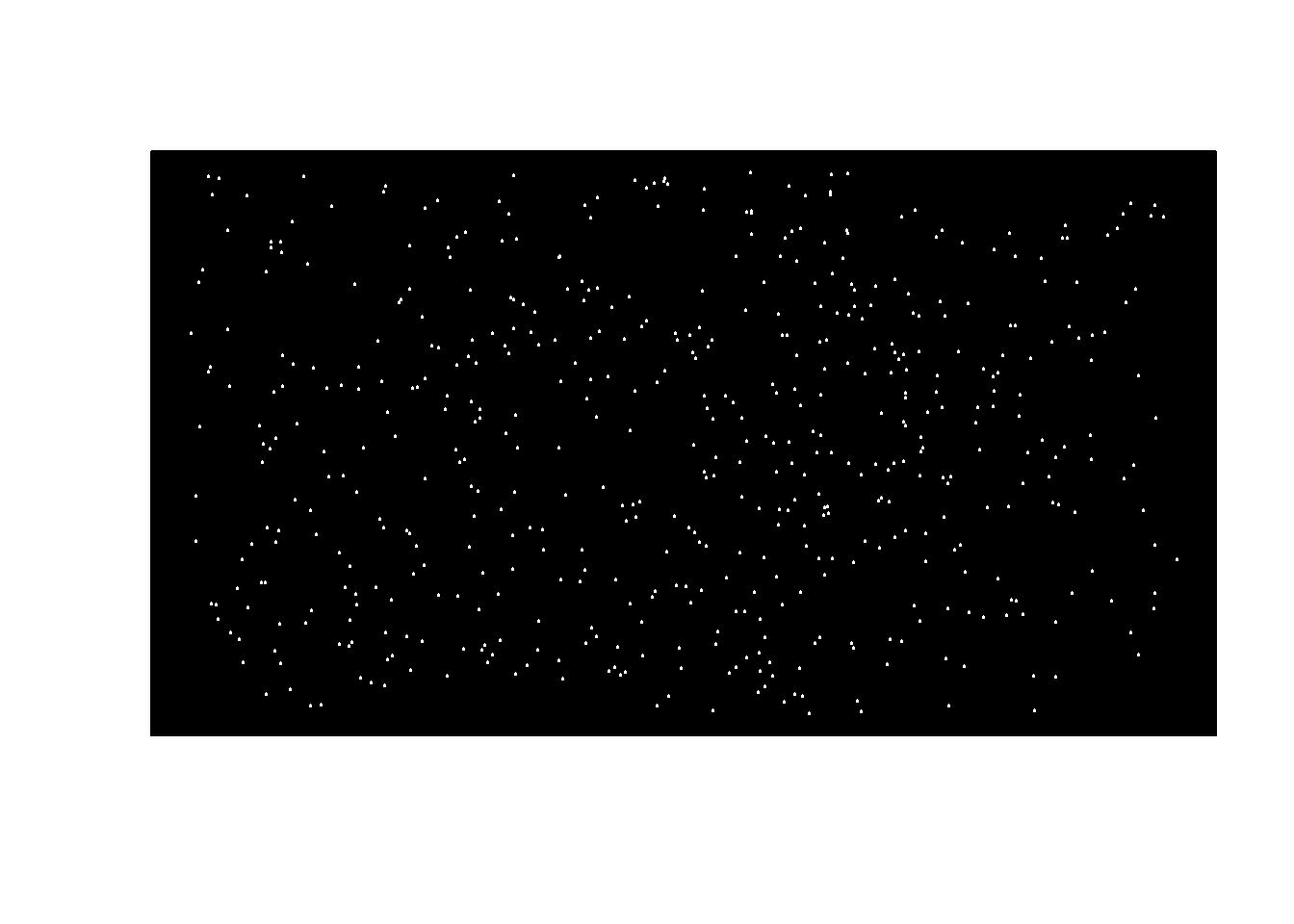
If only shown this picture, you might be hard-pressed to guess what the distribution refers to. That’s the beauty of statistics – the Poisson process can describe a range of wildly different phenomena that nevertheless share something fundamental in common. But while this sort of analysis is fun, it is worth remembering that these numbers have meaning through their connection to real events. Each data point signifies a real V-1 that was deliberately fired to kill civilians. We recommend reading some real memories from members of the public of that time, as archived by the BBC.
7 References
We have collected some references for further reading, including some which we weren’t able to include in our main article.
Aygin et al. (2019) Double cross: Geographic profiling of V-2 impact sites. Spatial Science. doi: 10.1080/14498596.2019.1642249
Clarke, R. D. (1946) An application of the Poisson distribution. Journal of the Institute of Actuaries, 72, 481. link
Evans, C. G and Delaney, K. B. (2018) The V1 (Flying Bomb) attack on London (1944–1945); the applied geography of early cruise missile accuracy Applied Geography 99:44-53 doi: 10.1016/j.apgeog.2018.07.019
Feller, W. (1950) An Introduction to Probability Theory and its Applications, Volume I. New York: John Wiley & Sons. pages discussing Clarke’s example
Franklin, C. (2010) Flying Bombs on London, Summer of 1944. link
Lidstone, G. I. (1942) Notes on the Poisson frequency distribution. Journal of the Institute of Actuaries, 71, 284– 291. link
Memories of V-1s and V-2s. WW2 People’s War. link
Presentation of an Institute Silver Medal to Mr. Roland David Clarke (1981). Journal of the Institute of Actuaries, 108, 7– 8. link
Pynchon, T. (1973) Gravity’s Rainbow. London: Cape. Amazon link
Ward, L. (2015) The London County Council Bomb Damage Maps 1939–1945. London: Thames & Hudson. Amazon link